The Simulated Annealing Algorithm
Written by Katrina Ellison Geltman on Thu 20 February 2014.
Simulated annealing is a method for finding a good (not necessarily perfect) solution to an optimization problem. If you're in a situation where you want to maximize or minimize something, your problem can likely be tackled with simulated annealing.
The traveling salesman problem is a good example: the salesman is looking to visit a set of cities in the order that minimizes the total number of miles he travels. As the number of cities gets large, it becomes too computationally intensive to check every possible itinerary. At that point, you need an algorithm.
Why choose simulated annealing?
There are many optimization algorithms, including hill climbing, genetic algorithms, gradient descent, and more. Simulated annealing's strength is that it avoids getting caught at local maxima - solutions that are better than any others nearby, but aren't the very best.
You can visualize this by imagining a 2D graph like the one below. Each x-coordinate represents a particular solution (e.g., a particular itinerary for the salesman). Each y-coordinate represents how good that solution is (e.g., the inverse of that itinerary's mileage).
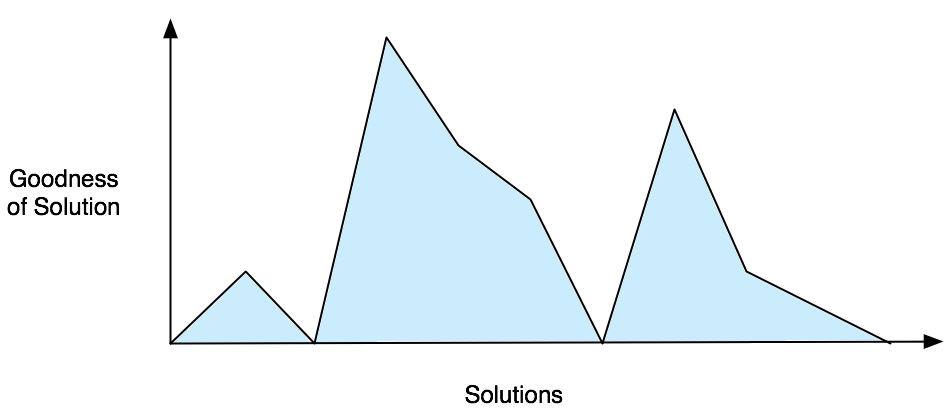
Broadly, an optimization algorithm searches for the best solution by generating a random initial solution and "exploring" the area nearby. If a neighboring solution is better than the current one, then it moves to it. If not, then the algorithm stays put.
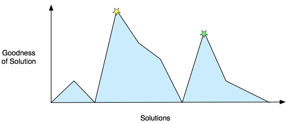
This is perfectly logical, but it can lead to situations where you're stuck at a sub-optimal place. In the graph below, the best solution is at the yellow star on the left. But if a simple algorithm finds its way to the green star on the right, it won't move away from it: all of the neighboring solutions are worse. The green star is a local maximum.
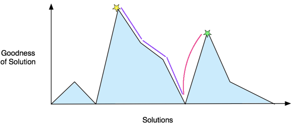
Simulated annealing injects just the right amount of randomness into things to escape local maxima early in the process without getting off course late in the game, when a solution is nearby. This makes it pretty good at tracking down a decent answer, no matter its starting point.
On top of this, simulated annealing is not that difficult to implement, despite its somewhat scary name.
The basic algorithm
Here's a really high-level overview. It skips some very important details, which we'll get to in a moment.
- First, generate a random solution
- Calculate its cost using some cost function you've defined
- Generate a random neighboring solution
- Calculate the new solution's cost
- Compare them:
- If cnew < cold: move to the new solution
- If cnew > cold: maybe move to the new solution
- Repeat steps 3-5 above until an acceptable solution is found or you reach some maximum number of iterations.
Let's break it down
First, generate a random solution
You can do this however you want. The main point is that it's random - it doesn't need to be be your best guess at the optimal solution.
Calculate its cost using some cost function you've defined
This, too, is entirely up to you. Depending on your problem, it might be as simple as counting the total number of miles the traveling salesman's traveled. Or it might be an incredibly complex melding of multiple factors. Calculating the cost of each solution is often the most expensive part of the algorithm, so it pays to keep it simple.
Generate a random neighboring solution
"Neighboring" means there's only one thing that differs between the old solution and the new solution. Effectively, you switch two elements of your solution and re-calculate the cost. The main requirement is that it be done randomly.
Calculate the new solution's cost
Use the same cost function as above. You can see why it needs to perform well - it gets called with each iteration of the algorithm.
If cnew < cold: move to the new solution
If the new solution has a smaller cost than the old solution, the new one is better. This makes the algorithm happy - it's getting closer to an optimum. It will "move" to that new solution, saving it as the base for its next iteration.
If cnew > cold: maybe move to the new solution
This is where things get interesting. Most of the time, the algorithm will eschew moving to a worse solution. If it did that all of the time, though, it would get caught at local maxima. To avoid that problem, it sometimes elects to keep the worse solution. To decide, the algorithm calculates something called the 'acceptance probability' and then compares it to a random number.
Those highly important details
The explanation above leaves out an extremely important parameter called the "temperature". The temperature is a function of which iteration you're on; its name comes from the fact that this algorithm was inspired by a method of heating and cooling metals.
Usually, the temperature is started at 1.0 and is decreased at the end of each iteration by multiplying it by a constant called $\alpha$. You get to decide what value to use for $\alpha$; typical choices are between 0.8 and 0.99.
Furthermore, simulated annealing does better when the neighbor-cost-compare- move process is carried about many times (typically somewhere between 100 and 1,000) at each temperature. So the production-grade algorithm is somewhat more complicated than the one discussed above. It's implemented in the example Python code below.
Example Code
This code is for a very basic version of the simulated annealing algorithm. A useful additional optimization is to always keep track of the best solution found so far so that it can be returned if the algorithm terminates at a sub- optimal place.
from random import random

def anneal(sol):
    old_cost = cost(sol)
    T = 1.0
    T_min = 0.00001
    alpha = 0.9
    while T > T_min:
        i = 1
        while i <= 100:
            new_sol = neighbor(sol)
            new_cost = cost(new_sol)
            ap = acceptance_probability(old_cost, new_cost, T)
            if ap > random():
                sol = new_sol
                old_cost = new_cost
            i += 1
        T = T*alpha
    return sol, cost
This skeleton leaves a few gaps for you to fill in: neighbor(), in which you
generate a random neighboring solution, cost(), in which you apply your cost
function, and acceptance_probability(), which is basically defined for you.
The acceptance probability function
The acceptance probability function takes in the old cost, new cost, and current temperature and spits out a number between 0 and 1, which is a sort of recommendation on whether or not to jump to the new solution. For example:
- 1.0: definitely switch (the new solution is better)
- 0.0: definitely stay put (the new solution is infinitely worse)
- 0.5: the odds are 50-50
Once the acceptance probability is calculated, it's compared to a randomly- generated number between 0 and 1. If the acceptance probability is larger than the random number, you're switching!
Calculating the acceptance probability
The equation typically used for the acceptance probability is:
$$ a = e^{\frac{c_{new} - c_{old}}{T}} $$
where $a$ is the acceptance probability, $(c_{new}-c_{old})$ is the difference between the new cost and the old one, $T$ is the temperature, and $e$ is 2.71828, that mathematical constant that pops up in all sorts of unexpected places.
This equation is the part of simulated annealing that was inspired by metalworking. Throw in a constant and it describes the embodied energy of metal particles as they are cooled slowly after being subjected to high heat. This process allows the particles to move from a random configuration to one with a very low embodied energy. Computer scientists borrow the annealing equation to help them move from a random solution to one with a very low cost.
This equation means that the acceptance probability:
-
is always > 1 when the new solution is better than the old one. Since you can't have a probability greater than 100%, we use $\alpha = 1$ in this case..
-
gets smaller as the new solution gets more worse than the old one.
-
gets smaller as the temperature decreases (if the new solution is worse than the old one)
What this means is that the algorithm is more likely to accept sort-of-bad jumps than really-bad jumps, and is more likely to accept them early on, when the temperature is high.
Conclusion
If you ever have a combinatorial optimization problem to solve, simulated annealing should cross your mind. Plenty of other strategies exist, but as algorithms expert Steven Skiena says, "[The] simulated annealing solution works admirably. It is my heuristic method of choice."
References
This post relies heavily on these notes from Graham Kendall at Nottingham University and on Steven Skiena's Algorithm Design Manual. Another excellent source is the 1983 paper "Optimization by Simulated Annealing" by Kirkpatrick, Gelatti, and Vecchi. It's a bit dense, but relatively readable for an academic paper.